The typical lifespan of software is much longer than hardware. It is important nowdays to consider a program’s scalability on multiple processor.

Amdahl’s Law is a famous equation that predicts the maximum theoretical speedup with additional processors.

The equation is simple to derive. It yields powerful yet pessimistic results.

I plotted the equation with some practical input to remind myself how poorly my code will scale in the future. 🙂

Equation

The idea is simple. Consider a computation that has three parts: setup, compute and finalize. The setup and finalize section can not be performed concurrently, but compute section can be parallelized to multiple processors.

The total running time given a number of processors would be the sum of three parts.

An important measurement is relative speedup. It that tells us how much faster the program is running with additional processors.

In a perfect world, if all parts of the computation can be performed concurrently, the speedup will be perfectly linear. This implies S(P) will always be the same as the number of processors. This is idealistic and highly unlikely in practice.

To find out the burden of the parts that can’t be parallelized, we first create a representation that describes them, denoted ɣ.

Now if we rewrite S(P) with ɣ, we will get Amdahl’s Law. This tells us that even if number of processor goes up infinitely, we are still bounded by 1/ɣ.

Efficiency, another metric, can be computed by normalizing S(P) by the number of processor.

Plots

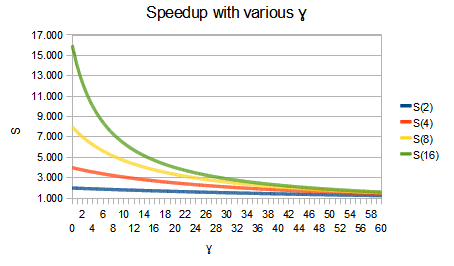
This plot shows the speedup on different ɣ value with 2,4,8 and 16 core scenario. From the graph, when ɣ is 50%, implying that 50% of the work can’t be parallelized, the increase in number of processor is nearly irrelevant.

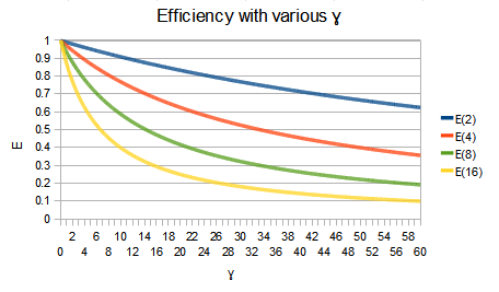
Efficiency is a metric that tells you if you are getting enough “bang for the buck” with more processors. As expected, efficiency curve drops more steeply as more cores are involved.

Pitfall

Amdahl’s Law assumes that the problem size stays fixed, and this is not always true. For example, if an application is to perform weather simulation, it is likely that an extra processor to add details to the model while the keeping the total execution time constant. If this is so, Amdahl’s law is more pessimistic than necessary.

This is a strong hint on how we can tackle the scalability problem in the future.

Conclusion

Pay attention to ɣ. If ɣ goes past 50%, the scalabilty outlook of the program is very poor.

Efficiency is important because it shows the law of diminishing on more processors.

Data

The plots and data can be downloaded here.